How to use Conditional Formatting in Excel

Microsoft is one of the most valuable tech companies in the world, with a market cap of over $3.2 trillion, ranking second to Apple, which has a market cap of slightly over $3.8 trillion. Excel is a spreadsheet application, owned and managed by Microsoft, for those who may not be familiar. This article contains a step-by-step guide on how to perform conditional formatting in Excel.

What is conditional formatting?

Conditional formatting is a powerful feature in Microsoft Excel that allows you to automatically apply formatting to cells based on their values. This functionality can help highlight important information, identify trends, and make your data easier to analyze.

Steps to Follow When Using Conditional Formatting

Step 1: Open Your Excel Workbook

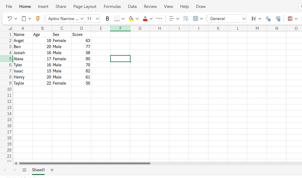
The first step is to open your excel workbook and ensure your data is clean, organized and ready for analysis.
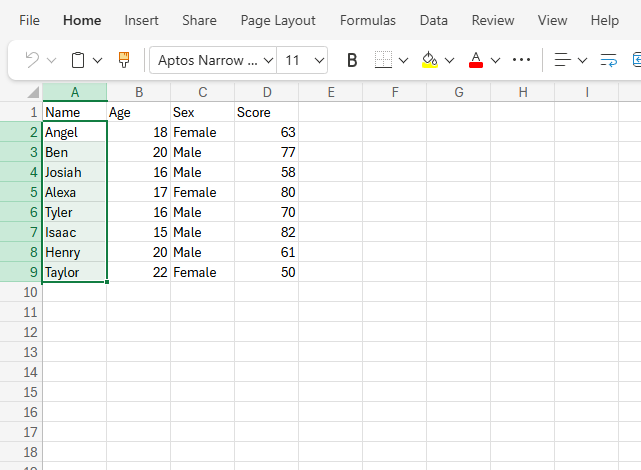
For example, you might have a table of sales figures, grades, or inventory levels. In this case we are working with a sample dataset.

Step 2: Select the Range of Cells

Highlight the range of cells where you want to format. For example, if you want to apply formatting to column A, click and drag to select the cells in that column

Step 3: Navigate the Conditional Formatting Menu

• Go to the Home tab on the Ribbon.
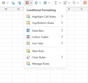
• In the Styles group, click on Conditional Formatting.

Step 4: Choose a Formatting Rule

Excel provides several predefined rules for conditional formatting. You can choose from the following options:

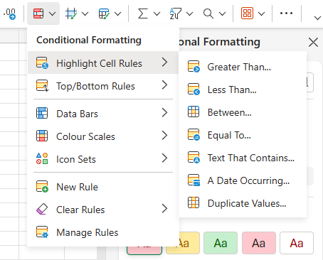
1. • Highlight Cell Rules: Use this to format cells based on comparisons, such as greater than, less than, or equal to specific values. You can also highlight duplicated values and texts with certain letters in them.
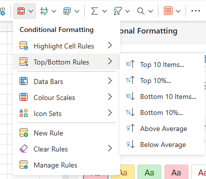
   • Top/Bottom Rules: Highlight the top 10% or bottom 10% of values, or other metrics.
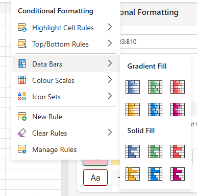
   • Data Bars: They add a gradient or solid fill inside cells to represent those which meet the condition set.
   • Color Scales: Apply a range of colors based on the cell values.
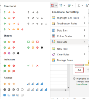
   • Icon Sets: Display icons within cells based on the set rule.                                          

Step 6: Apply a rule

• Select a rule from the menu. For example, choose Highlight Cells Rules > Greater Than….
• In the dialog box, specify the condition and formatting. For instance, type “500” to highlight cells with values greater than 500.
• Choose a formatting style (e.g., fill color, font color) from the dropdown or click Custom Format to create your own.
• Click OK to apply the rule.

Once you’ve selected a rule Excel will automatically apply it to the selected range. Review the results to ensure the formatting aligns with your intent.

Take the next step toward mastering conditional formatting

Step 7: Manage and Clear Rules

To adjust or remove conditional formatting:

• Go to Conditional Formatting > Manage Rules…
• In the Conditional Formatting Rules Manager, select the rule you want to modify and click Edit Rule or Delete Rule.

To create a new rule:

• Click on the Conditional Formatting menu.
• Select New Rule to create a rule suitable for your analysis.
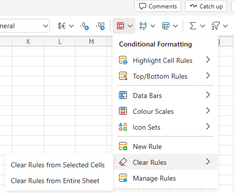
• Use Clear Rules to remove all formatting from a selection or the entire worksheet

Practical Use Cases for Conditional Formatting

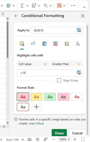
Example: Highlight ages above 18

• Select the Age data column.

• Go to Home > Conditional Formatting > Highlight Cells Rules > Greater Than…

• Enter “18” and choose a red fill.

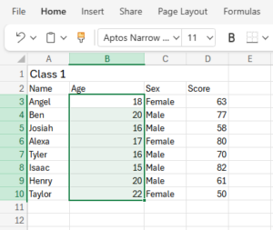
Example 2: Duplicated ages can also be located with conditional formatting.

• Select the column with duplicated values (age column)

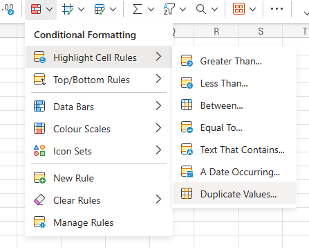
• Go to Home > Conditional Formatting > Highlight Cell Rules> Duplicate Values…

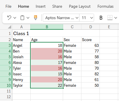
• All duplicates are highlighted in red fill

Conclusion

In this article, we explored the concept of conditional formatting in Excel. Overall, conditional formatting is a powerful and versatile tool that can significantly enhance your data analysis skills. By applying the steps outlined, you can use this feature to uncover valuable insights and present your data in a more visually compelling way.